Linkages geometry with GeoGebra and LEGO
by Zoltán Kovács
Abstract
A basic task of engineering is the problem of
assembling mechanisms that make an element move along a
prescribed path. In the modern era many applications still rely on
classic methods that use belts, chains, ball bearings or shafts—all
of these applications can be well modeled by mathematical means.
In the talk we focus on mathematical modeling of mechanical
engineering by using computer algebra for calculation and
a LEGO compilation for supplementary experiments. We discuss
some novel methods in the dynamic geometry software GeoGebra Discovery
to study the motion of linkages from both the computation and
the experimental views at the same time.
What is a mechanical linkage?
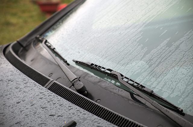
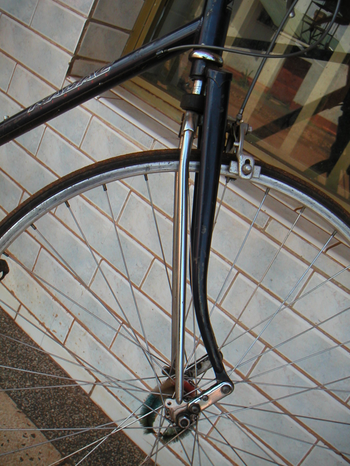

Example: Bike reflector (tracing the cat's eye)
Constructing linkages that are based on algebraic setups
Algebraic: only polynomial equations with integer coefficients are allowed.
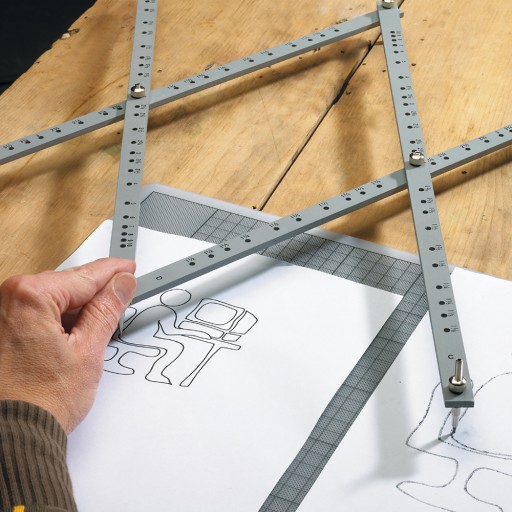
The simplest setup: a compass
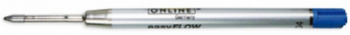
All you need to draw a circle are: a sheet of paper and a G2 pen refill.
In fact, the drawn curve will be an incomplete circle, but always consider
the Zariski closure of the appearing object.
Setup #2: a finger
This construction is not very useful. In fact, you should be able to draw a region of points.
A so-called 3-bar linkage is therefore does not result in a solid curve.
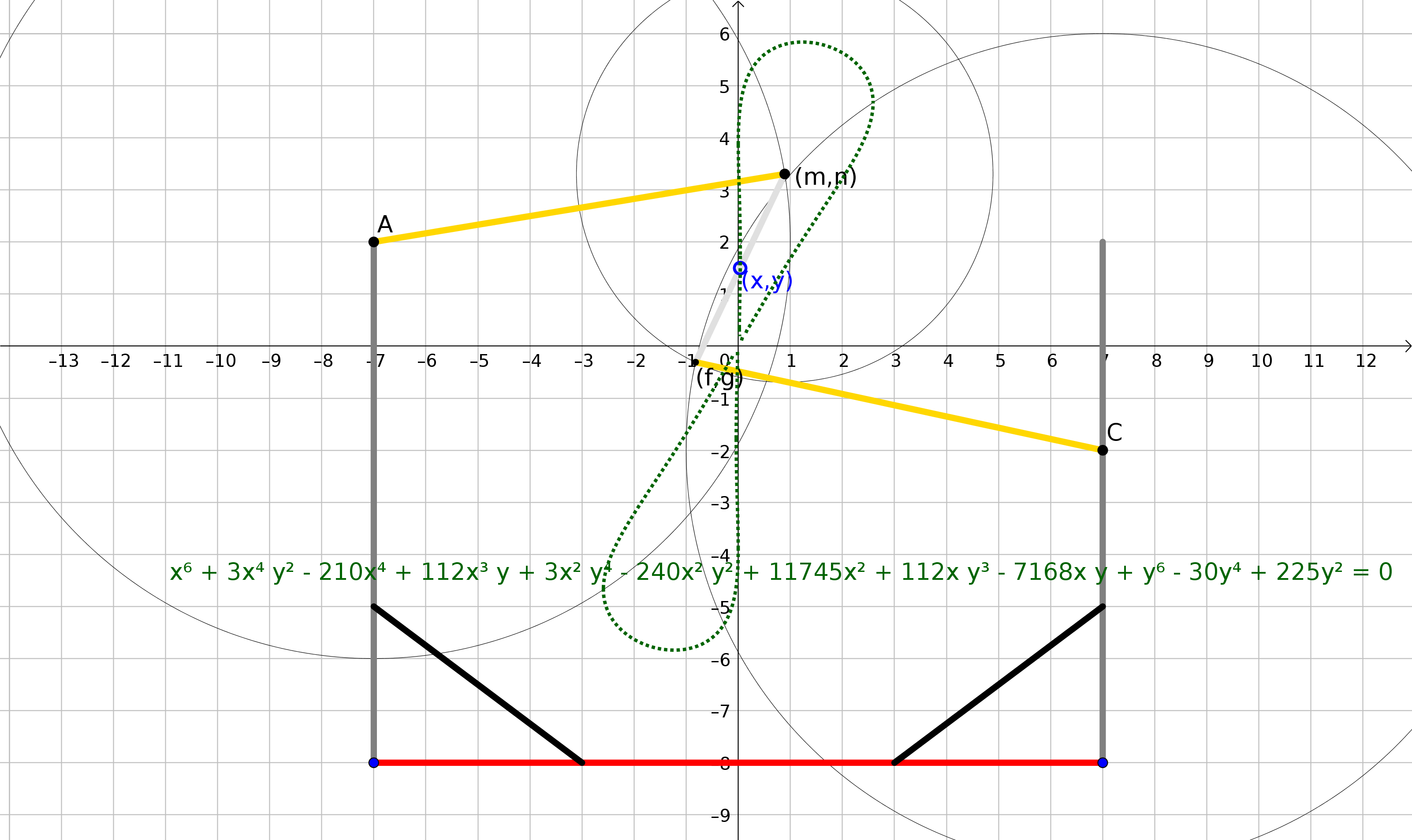
Setup #3: A 4-bar linkage
So it seems to make more sense to add another bar and close the linkage. The gray bars would provide only
circular shapes, but interestingly, all three inner positions of the white beam result in a non-exact circular arc.
When the grey bars show this crossed form and the pen refill is in the midpoint of the white beam, the obtained
curve seems linear. This situation should be investigated by using more accurate means!
Since this is an algebraic situation, the algebraic equation of the drawn curve can be explicitly computed
by an efficient algorithm:
\[x^6-24x^5+\ldots=\ldots\]
One can show (either experimentally, numerically or symbolically) that any part of the curve is neither an arc of a regular circle,
nor a segment of a completely straight line. In fact, it is a sextic (a degree 6 polynomial) which plays an
important role when describing 4-bar linkages.
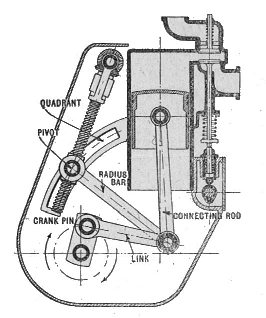
Setup #4: Another 4-bar linkage: Watt's steam machine
We can compute this curve with GeoGebra by describing the situation step-by-step
with algebraic translation.
Now type Eliminate({$1, $2, $3, $4, $5}, {f, g, m, n}) to get a list
of equations that faithfully describe the situation after eliminating the unnecessary variables.
The result, in our case, is a single element which is, again, a sextic!
I feel uneasy when facing sextics – is not there something simpler?
The good news: there is, the ellipsograph (setup #5)
Now you may want to play with the parameters. By dragging the sliders you can learn that
the obtained formula is always an ellipse:
\[x^2+\ldots\]
How to create such applets in GeoGebra?
| No. | Name | Toolbar Icon | Description | Definition | Value |
|---|---|---|---|---|---|
| 2 | Number l | l = 4 | |||
| 3 | Point A | Point on xAxis | Point(xAxis) | A = (-1.33, 0) | |
| 4 | Circle c | Circle with center A and radius l | Circle(A, l) | c: (x + 1.33)² + y² = 16 | |
| 5 | Number r | r = 14 | |||
| 6 | Point B | Intersection of c and yAxis | Intersect(c, yAxis, 1) | B = (0, 3.77) | |
| 7 | Line f | Line A, B | Line(A, B) | f: -3.77x + 1.33y = 5.02 | |
| 8 | Point C | B dilated by factor r / l from A | Dilate(B, r / l, A) | C = (3.33, 13.2) | |
| 11 | Implicit Curve eq1 | LocusEquation(C, A) | LocusEquation(C, A) | eq1: 49x² + 25y² = 4900 | |
| 12 | Segment g | Segment C, A | Segment(C, A) | g = 14 |
To simplify things, we skipped steps 1, 9 and 10 (and some later ones that do fancy details). Power users may want to learn how
the overrun handling is implemented by downloading the applet and open it in
GeoGebra Discovery after installing the program.
(There is some JavaScript knowledge required.)
We emphasize that it is quite easy to create a minimal version of this applet. In fact, steps 7 and 12 do not play any role in
the computation. Also, steps 2 and 5 help only in the generalization of the problem. That is, at the end of the day,
one needs only the following steps to create the simplest version of the applet:
| No. | Name | Toolbar Icon | Description | Definition | Value |
|---|---|---|---|---|---|
| 3 | Point A | Point on xAxis | Point(xAxis) | A = (-1.33, 0) | |
| 4 | Circle c | Circle with center A and radius l | Circle(A, 4) | c: (x + 1.33)² + y² = 16 | |
| 6 | Point B | Intersection of c and yAxis | Intersect(c, yAxis, 1) | B = (0, 3.77) | |
| 8 | Point C | B dilated by factor 14 / 4 from A | Dilate(B, 14 / 4, A) | C = (3.33, 13.2) | |
| 11 | Implicit Curve eq1 | LocusEquation(C, A) | LocusEquation(C, A) | eq1: 49x² + 25y² = 4900 |
Exercises
- Prove that the Chebyshev curve does not contain any exactly linear segments on its quasi-linear part. (Use reductio ad absurdum and the fact that a polynomial equation has a finite number of solutions.)
- Prove the same for Watt's curve.
- Find some configurations of a 4-bar linkage that result in multiple curves, e.g. a conic and a quartic. (Use factorization to check that the curves are different algebraically, not just geometrically. Explain the difference by using the case of a hyperbola and its branches.)
- Is it possible to create a 4-bar linkage whose movement corresponds to exactly three curves, namely, three circles? If yes, how?
- For which parameters can we obtain a circle in setup #5? Prove your conjecture by using Thales' circle theorem.
- By using the previous exercise, generalize your result by using stretching and show that the ellipsograph indeed produces an ellipse.
- Build Chebyshev's lambda linkage – both as a LEGO construction and also as a GeoGebra applet. Prove that it produces the same curve as the above mentioned one.
- Build Hart's inversor and Hart's A-frame. Prove that they produce straight lines. (Use factorization after elimination.)
- Try the A2 pen refill by building some additional linkages shown on the GitHub page lego-linkages. In particular, build Peaucellier's linkage as another example to establish a straight linear motion.
- Prove that Peaucellier's linkage produces a straight linear motion. Use elimination or geometric inversion.
References
- Lindner, A.: The trace of reflectors as a roulette. 2015. (First appearance in German as Die Spur von Katzenaugen. 2014. An updated version can be found as Die Spur von Reflektoren als Rollkurve. 2015.) )
- Bryant, J. and Sangwin, C.: How round is your circle? Where engineering and mathematics meet. Princeton, New Jersey: Princeton University Press. 2008.
- Vincent, J.: Dynamic Geometry Software and Mechanical Linkages. In Networking the Learner: Computers in Education, Watson, D. and Andersen, J., Editors. Springer, Boston, MA. p. 423–432. 2002.
- Kempe, A. B.: How to draw a straight line: A lecture on linkages. London, Macmillan. 1877.
- Kovács, Z. and Kovács, B.: A compilation of LEGO Technic parts to support learning experiments on linkages.
- Kovács, Z. and Jodlbauer, S.: Ellipsograph of Archimedes as a simple LEGO construction. 2020.
- Kovács, Z., Recio, T. and Vélez, M. P.: Using Automated Reasoning Tools in GeoGebra in the Teaching and Learning of Proving in Geometry. International Journal of Technology in Mathematics Education, 25 p. 33–50. 2018.
- Kovács, Z., Recio, T. and Vélez, M. P.: Reasoning about linkages with dynamic geometry. Journal of Symbolic Computation. 2019.
- Kovács, Z.: Motion with LEGOs and Dynamic Geometry. Virginia Mathematics Teacher Journal, 44 p. 43–48. 2018.
- Kovács, Z.: Physical and virtual linkages. YouTube video. 2019.
- Kovács, Z.: A LEGO kit for prospective math teachers. 2022.
Acknowledgements
The author was partially supported by a grant
PID2020-113192GB-I00 from the Spanish MICINN.

|
Zoltán Kovács Linz School of Education Johannes Kepler University Altenberger Strasse 69 A-4040 Linz |